Using the FAµST Factorization Wrappers
Previous live scripts already addressed a part of the matfaust's functionalities however matfaust.fact which is a central module was not covered. It is mainly dedicated to the algorithms that (approximately) factorize a dense matrix into a Faust object. This is the subject covered (partly) in this live script.
You will see how to launch the algorithms easily, how to feed them with your own complex set of parameters, how to run them for only few steps when possible, how to use a variant or another, how to enable debugging information, etc.
Table of Contents
1. The Hierarchical PALM4MSA Algorithm
1.1 Generating a Hadamard Matrix
Before to tackle Hadamard matrices factorization, let's introduce one matfaust's function which is actually directly related: wht.
This method allows you to generate sparse Hadamard transforms.
import matfaust.wht
% generate a Hadamard Faust of size 32x32
FH = wht(32, false); % normed=false is to avoid column normalization
H = full(FH); % the dense matrix version
imagesc(FH)

numel(nonzeros(H))
ans = 1024
All the factors are the same, let's print the first one.
figure()
imagesc(full(factors(FH, 1)))

You might want to verify if H is a proper Hadamard matrix.
is_hadamard = true;
mats = {H, H.'};
for m=1:2
H_ = mats{m};
for i=1:size(H_, 1)-1
for j=i+1:size(H_, 1)
is_hadamard = is_hadamard && all(H_(i,:)*H_(j,:).' == 0);
end
end
end
[~, ~, nz] = find(H); % all nonzeros of H in nz
is_hadamard = is_hadamard && all(abs(nz) == 1)
The code above basically verifies that all column or row vectors are mutually orthogonal and made only of -1, 0 and 1 coefficients, that is exactly the Hadamard matrix definition. The response is yes, so we can go ahead.
1.2 Factorizing a Hadamard Matrix
Let's begin by factorizingHthe easy way with the automatic parametrization provided by matfaust.
import matfaust.faust_fact
FH2 = faust_fact(H, 'hadamard')
imagesc(FH2)

Interestingly, the FH2's factors are not the same as FH's but the resulting full array is exactly the same. Just to be sure let's verify the relative error against H.
err = norm(FH2-H)/norm(H)
err = 2.7128e-15
Good!
The argument 'hadamard' of faust_fact is a shorthand to a set of parameters fitting the factorization of Hadamard matrices.
Speaking about shorthand, faust_fact is an alias of matfaust.fact.hierarchical. This function implements the hiearchical factorization based on PALM4MSA. For details about the theory behind these algorithms you can read Luc Le Magoarou's thesis manuscript.
We won't go into further details nevertheless it's important to see how to define the parameters manually in order to proceed to your own custom factorizations. For that purpose we need to describe approximately the algorithm but please keep in mind this is just an insight (for instance, the norms below are voluntarily not defined).
Basically, the hierarchical algorithm works like this:
- If you want to decompose a matrixMin J factors, the algorithm will iterate
 times. Each iteration follows two steps:
1. (local optimization) At each iteration  , the currently considered matrix
  (with
(with  ) is decomposed in two factors by the PALM4MSA algorithm as respect to the minimization of
  .
.
2. (global optimization) At the end of each iteration i, PALM4MSA is called again to ideally compute the 
- So ideally at the end of the iteration you'll get something like
 taking
  .
.
1.2.1 Defining the Constraints
The explanation above is eluding something essential: the sparsity constraints. Indeed, the purpose of the algorithm is not only to decompose a matrix but moreover to enhance its sparsity, as hinted by the FAµST acronym: Flexible Approximate Multi-layer Sparse Transform.
So you'll need to feed the algorithm with sparsity constraints. In fact, you'll define one pair of constraints per iteration, the first is for  (the main factor) and the second for
  (the residual).
The matfaust API is here to help you define the constraints in one shot but you can if you want define constraints one by one as we'll see later.
Let's unveil the factorization constraints to decompose the Hadamard matrix .
.
Let's go back to the code and define our constraints as lists (provided by the module matfaust.factparams):
import matfaust.factparams.ConstraintList
n = size(H, 1);
S_constraints = ConstraintList('splincol', 2, n, n, ...
'splincol', 2, n, n, ...
'splincol', 2, n, n, ...
'splincol', 2, n, n);
R_constraints = ConstraintList('splincol', n/2, n, n, ...
'splincol', n/4, n, n, ...
'splincol', n/8, n, n, ...
'splincol', n/16, n, n);
The 'splincol' constraint used here is for defining the maximum number of nonzeros elements to respect for any row or column of the considered matrix (here or ). Looking at S_constraints initialization, we see in the first line 'splincol', 2, n, n; the value 2 means we target 2 nonzeros per-column and per-row, the next arguments define the size of the matrix to constrain (its number of rows and columns).
So in the example of S_constraints all the targeted matrices have 2n nonzeros.
More generally in matfaust, the constraints are defined in terms of norms, in our case of Hadamard factorization we used 0-norm (which is not actually a norm) as follows:
Enough of explanations! I let you decrypt why R_constraints correspond likewise to (C2).
But wait a minute, what would happen if we have a set of one hundred constraints? Don't worry! The matfaust API allows to alternatively set the constraints one by one:
import matfaust.factparams.ConstraintInt
S_constraints = {};
R_constraints = {};
for i=1:4
S_constraints = [ S_constraints {ConstraintInt('splincol', n, n, 2)} ];
R_constraints = [ R_constraints {ConstraintInt('splincol', n, n, n/2^i)}];
end
S_constraints and R_constraints are still the exact same set of constraints as before.
ConstraintInt is a family of integer constraints. More globally, there is a hierarchy of classes whose parent class is ConstraintGeneric where you'll find other kind of constraints ; ConstraintMat, ConstraintReal.
The table here can give you an idea of each constraint definition. Most constraints are associated to a proximal operator which projects the matrix into the set of matrices defined by the constraint or at least it tries to (because it's not necessarily possible).
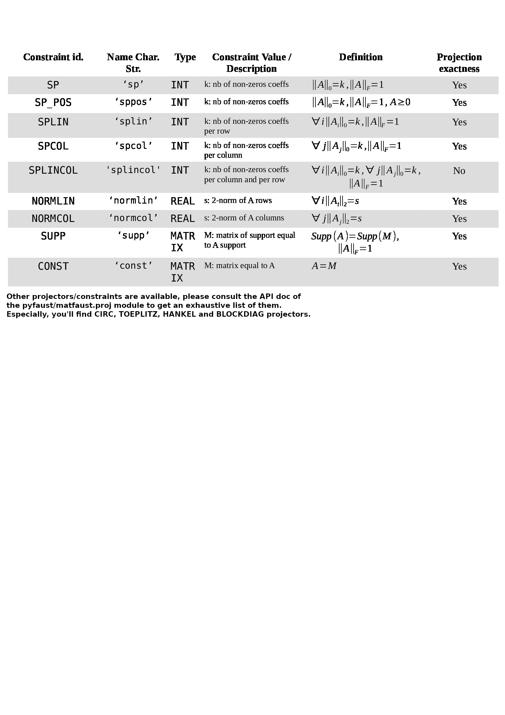
In the latest version of FAµST it's possible to project matrices from the wrappers themselves, let's try one ConstraintInt:
import matfaust.factparams.ConstraintInt
A = rand(10, 10);
A_ = ConstraintInt('sp', 10, 10, 18).project(A);
Annz = numel(nonzeros(A))
Annz = 100
A_nnz = numel(nonzeros(A_))
A_nnz = 18
We asked for a sparsity of 18 nonzeros and that's what we got after calling project.
The function project can help you debug a factorization or even understand exactly how a prox works for a specific constraint and matrix.
Another API doc link completes the definition of constraints : ConstraintName
If you find it complicated to parameterize your own set of constraints, well, you are not the only one! You may be happy to know that it is one of the priorities of the development team to provide a simplified API for the factorization algorithms in an upcoming release.
A simplification is already available with the pyfaust.proj package for which you might read the following specific notebook: Using The FAµST Projectors API. An example of the same configuration of constraints but the projector way is introduced in 1.2.3.
1.2.2 Setting the Rest of the Parameters and Running the Algorithm
OK, let's continue defining the algorithm parameters, the constraints are the most part of it. You have optional parameters too, but one key parameter is the stopping criterion of the PALM4MSA algorithm. You have to define two stopping criteria, one for the local optimization and another for the global optimization.
import matfaust.factparams.StoppingCriterion
loc_stop = StoppingCriterion('num_its', 30);
glob_stop = StoppingCriterion('num_its', 30);
The type of stopping criterion used here is the number of iterations of PALM4MSA, that is the number of times all the current factors ( included) are updated either for the local or the global optimization. So, with the initialization of loc_stop and glob_stop above, if you ask J factors (through the number of constraints you set) you'd count a total of  iterations of PALM4MSA.
Ok, I think we're done with the algorithm parameters, we can pack them into one object and give it to faust_fact.
import matfaust.factparams.ParamsHierarchical
params = ParamsHierarchical(S_constraints, R_constraints, loc_stop, glob_stop, 'is_update_way_R2L', true); % the argument order matters!
% launch the factorization
FH3 = faust_fact(H, params)
err = norm(FH3-H)/norm(H)
err = 2.7128e-15
You might wonder what is the boolean is_update_way_R2L. Its role is to define if the PALM4MSA algorithm will update the and last factors from the left to right (if false) or toward the opposite direction (if true). It does change the results of factorization!
I must mention that there are several other optional arguments you'd want to play with for configuring, just dive into the documentation.
You also might call the PALM4MSA algorithm directly (not the hierarchical algorithm which makes use of it), the function is here. You can theoretically reproduce the hierarchical algorithm step by step calling palm4msa() by yourself.
Well, there would be a lot to say and show about these two matfaust algorithms and their parameters but at least with this example, I hope, you got an insight of how it works.
1.2.3 Using Projectors instead of ConstraintList-s
Now that we know how to factorize a matrix, let's show in this short section how to use a more handy matfaust API component than ConstraintList to define a set of projectors (or proximity operators) instead of constraints. Indeed when a Constraint* object is defined behind the scene a projector is used to compute the matrix image (with respect to a certain structure, e.g. the sparsity of the matrix). So why don't we directly define projectors? That is the thing, there is no reason not to do that, moreover it's simpler! So let's see how to define the Hadamard matrix factorization set of projectors and run again the algorithm.
import matfaust.proj.*
S_projs = {};
R_projs = {};
for i=1:4
S_projs = [ S_projs {splincol(size(H), 2)}];
R_projs = { R_projs {splincol(size(H), n/2^i)}};
end
params = ParamsHierarchical(S_constraints, R_constraints, loc_stop, glob_stop, 'is_update_way_R2L', true); % the argument order matters!
% launch the factorization
FH4 = faust_fact(H, params)
err = norm(FH4-H)/norm(H)
err = 2.7128e-15
As you see the factorization gives exactly the same Faust as the one before (with ConstraintList instead of matfaust.proj list). It could seem to be just a syntactic detail here to use the matfaust.proj package instead of ConstraintList but it is more than that, projectors like splincol are functors and can be used easily to project a matrix.
Again, I can only advise you to read the dedicated live script about projectors if you want to go further into details about projectors and discover the collection of the projectors available in the matfaust API.
Since version 2.4, FAµST is able to compute Fast Graph Fourier Transforms. Indeed, FAµST includes the Truncated Jabcobi Algorithm algorithm for this goal. It allows to diagonalize symmetric positive definite matrices.
2. The GFT Algorithm
It is implemented in C++ and a Python wrapper make it available from pyfaust.
Here again the theory isn't what matters but feel free to take a look at the following papers:
- Le Magoarou L., Gribonval R., Tremblay N., “Approximate fast graph Fourier transforms via multi-layer sparse approximation“,Transactions on Signal and Information Processing over Networks
- Le Magoarou L. and Gribonval R., "Are there approximate Fast Fourier Transforms on graphs ?", ICASSP, 2016
2.1 The Truncated Jacobi Algorithm
Let's run the truncated Jacobi algorithm for eigen decomposition, hence the name eigtj, on a random Laplacian example. You'll see it's really straightforward!
import matfaust.fact.eigtj
n = 2500;
% Let's try to diagonalize a random Laplacian
Lap = sprand(n, n, .001);
Lap = full(tril(Lap)+tril(Lap)');
[Uhat, Dhat] = eigtj(Lap, 'tol', . 3); % targeted relative error of 0.09
Now verify the error asked is really what we finally get:
err = norm(Uhat*Dhat*Uhat'-Lap, 'fro')/norm(Lap, 'fro')
err = 0.2998
Write some code to check the first factor of  is orthogonal and then that itself is orthogonal (with a tolerance near to the machine espilon).
Uhat0 = factors(Uhat, 1);
n = size(Uhat, 1);
all(all(full(Uhat0*Uhat0') - eye(n) < 10^-12))
norm(Uhat*Uhat' - eye(n))
ans = 5.5411e-16
Yes it is definitely orthogonal.
As you saw above the error err is quite good but you really can tune the algorithm to achieve a specific tradeoff between accuracy and sparsity. It's time to read the documentation, you'll learn about the maybe most important of eigtj which is 'nGivens'.
Is that all? No, we can evaluate the memory saving brings as a Faust relatively to the matrix U obtained by Matlab's eig().
[U, D] = eig(Lap);
err2 = norm(U*D*U'-Lap)/norm(Lap)
err2 = 7.5968e-15
nnz_sum(Uhat)
ans = 54928
numel(nonzeros(U))
ans = 6111748
The memory space to store is smaller since its number of nonzeros elements is less than that of U.
x = rand(n, 1);
timeit(@() Uhat*x)
ans = 0.0012
timeit(@() U*x)
ans = 0.0155
The execution time for Faust-vector multiplication is really better too (compared to the matrix-vector multiplication) ! Applying the Graph Fourier Transform on x is faster.
The third live script is ending here, I hope you'll be interested to dig into matfaust API and maybe even give some feedback later. The API has made a lot of progress lastly but it remains a work-in-progress and some bugs might appear here or there. Besides, the documentation and the API can always receive some enhancement so don't hesitate, any suggestion is welcome!
Note: this livescript was executed using the following matfaust version:
matfaust.version()